


Process Validation
Latest News
Advertisement
Latest Videos

Advertisement
More News

Understanding processes in the development and manufacture of biological drug substances is crucial to successfully navigating the clinical phases towards commercial launch, all within ever‑tightening time constraints, and regulatory frameworks.

This article focuses on drawing parallels between ICH Q14/Q2(R2), United States Pharmacopeia (USP) <1220>, and International Organization for Standardization/International Electrotechnical Commission (ISO/IEC) 17025:2017.

This article provides an overview of validation concept principles evolution to a life cycle risk-based approach with focus on compendial perspectives.
Process validation for a drug product must be done with commercial scale batches, says Siegfried Schmitt, vice president, Technical at Parexel.
Experts Susan J. Schniepp, distinguished fellow for Regulatory Compliance Associates, and Steven J. Lynn, executive vice-president, Pharmaceuticals for Regulatory Compliance Associates, discuss the verification of compendial methods.

Qualified algorithms enable validation of machine learning models that can be used for process optimization.
Genezen has opened its new process development and analytical lab for viral vector production.

The benefits of single-use technologies for upstream viral-vector processes clearly outweigh their disadvantages.

A structured assessment process can determine compliance to lifecycle process-validation requirements for biopharmaceuticals.

The industry is moving beyond cleaning’s “low tech” image to embrace science-based limits and statistical approaches to control.

AFI representatives of the process validation working group explore and define key elements for an enhanced approach to process validation for sterile liquid and freeze-dried forms.
The European Directorate for the Quality of Medicines and Healthcare (EDQM) has published a new general chapter (2.6.32) in the European Pharmacopoeia (Ph. Eur.) supplement 10.3.
The company now offers its CONFIDENCE virus clearance services to support validation of viral clearance processes.

Experience, communication, collaboration, transparency, planning, and prioritization contribute to success.

While cell and gene therapies differ in many ways, some of the best practices for process development and validation are similar.

Getting the science right helps biopharma startups overcome development and commercialization challenges.
A properly designed validation program will detect variation and ensure control based on process risk.

This study was successful in establishing a reliable and effective method for evaluating cleaning processes based on risk. Click here to view a PDF of this article.
Managing data at the different stages of the lifecycle, linking disparate systems together, and making the right data available to those who need it is problematic and time consuming.

A validation plan developed to support a process unrelated to bio- pharmaceutical manufacture is applied to bio- pharmaceutical processes and systems.
Process understanding and careful assessment of risks are essential in developing viral clearance programs.
This is the first of a series of three articles about validation and technical transfer in the bio- pharmaceutical industry.

Process validation is an extension of biologics development processes.
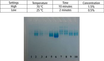
This article demonstrates that a modified SDS–PAGE can be easily used as a tool for quantifying the degree of protein degradation.

Rinse sample analysis or visual inspection are risk-based approaches that can be correlated to surface cleanliness to replace surface sampling in a biopharmaceutical equipment cleaning process.
Advertisement
Advertisement